How to explore to find a robust control policy?

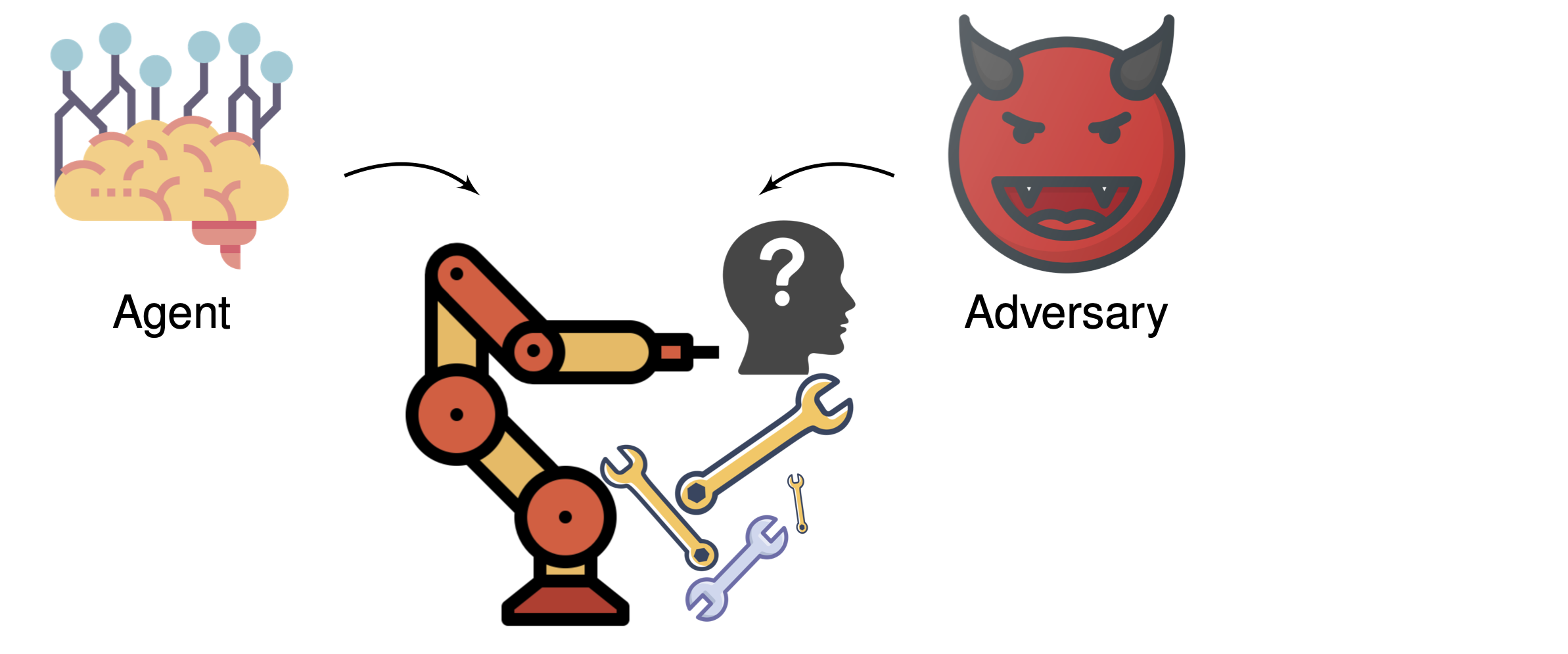
Figure 1: We propose an algorithm that learns a policy for continuous control tasks even when a worst-case adversary is present.

This is a post for the work Combining Pessimism with Optimism for Robust and Efficient Model-Based Deep Reinforcement Learning (Curi et al., 2021), jointly with Ilija Bogunovic and Andreas Krause, that appeared in ICML 2021. It is a follow-up on Efficient Model-Based reinforcement Learning Through Optimistic Policy Search and Planning (Curi et al., 2020), that appeared in NeuRIPS 2020 (See blog post)

Introduction

In this work, we address the challenge of finding a robust policy in continuous control tasks. As a motivating example, consider designing a braking system on an autonomous car. As this is a highly complex task, we want to learn a policy that performs this maneuver. One can imagine many real-world conditions and simulate them during training time e.g., road conditions, brightness, tire pressure, laden weight, or actuator wear. However, it is unfeasible to simulate all such conditions and that might also vary in potentially unpredictable ways. The main goal is to learn a policy that provably brakes in a robust fashion so that, even when faced with new conditions, it performs reliably.

Of course, the first key challenge is to model the possible conditions the system might be in. Inspired by $\mathcal{H}_\infty$ control and Markov Games, we model unknown conditions with an adversary that interacts with the environment and the agent. The adversary is allowed to execute adversarial actions at every instant by observing the current state and the history of the interaction. For example, if one wants to be robust to laden weight changes in the braking example, we allow the adversary to choose the laden weight. By ensuring good performance with respect to the worst-case laden weight that an adversary selects, then we may also ensure good performance with respect to any other laden weight. Consequently, we say that such policy is robust.

The main algorithmic procedure is to train our agent together with a fictitious adversary that simulates the real-world conditions we want to be robust to. The key question we ask is: How to train these agents in a data-efficient way?. A common procedure is domain randomization (Tobin et al., 2020), in which the adversary is simulated by sampling at random from a domain distribution. This has proved useful for sim2real applications, but it has the drawback that it requires many domain-related samples, as easy samples are treated equally than hard samples, and it scales poorly with the dimensionality of the domain. Another approach is RARL (Pinto et al., 2017), in which the adversary and the learner are trained with greedy gradient descent, i.e., without any exploration. Although RARL performs well in some tasks, we demonstrate that the lack of exploration, particularly by the adversary, yields poor performance.

Problem Setting

In this section, we formalize the ideas from the introduction. We consider a stochastic environment with states $s$, agent actions $a$, adversary actions $\bar{a}$, and i.i.d. additive transition noise vector $\omega$. The dynamics are given by:

$$\begin{align} s_{h+1} = f(s_h, a_h, \bar{a}_h) + \omega_h \end{align}$$

We assume the true dynamics $f$ are unknown and consider the episodic setting over a finite time horizon $H$. After every episode (i.e., every $H$ time steps), the system is reset to a known state $s_0$. At every time-step, the system returns a reward $r(s_h, a_h, \bar{a}_h)$. We consider time-homogeneous agent policies $\pi$, that select actions according to $a_h = \pi(s_h)$, as well as adversary policies $\bar{\pi}$ with $\bar{a}_h = \bar{\pi}(s_h)$. We consider the performance of a pair of policies $(\pi, \bar{\pi})$ on a given dynamical system $\tilde{f}$ as the episodic expected sum of returns:

$$\begin{align} J(\tilde{f}, \pi, \bar{\pi}) &:= \mathbb{E}_{\tau_{\tilde{f}, \pi, \bar{\pi}}}{ \left[ \sum_{h=0}^{H} r(s_h, a_h, \bar{a}_h) \, \bigg| \, s_0 \right]}, \quad \text{s.t. Eq.(1).} \end{align}$$

where $\tau_{\tilde{f},\pi,\bar{\pi}}$ is a random trajectory induced by the stochastic noise $\omega$, the dynamics $\tilde{f}$, and the policies $\pi$ and $\bar{\pi}$.

We use $\pi^{\star}$ to denote the optimal robust policy from the set $\Pi$ on the true dynamics $f$, i.e.,

$$\begin{align} \pi^\star \in \arg \max_{\pi \in \Pi} \min_{\bar{\pi} \in \bar\Pi} J(f, \pi, \bar\pi). \end{align}$$

For a small fixed $\epsilon>0$, the goal is to output a robust policy $\hat{\pi}_{T}$ after $T$ episodes such that:

$$\begin{align} \min_{\bar{\pi} \in \bar{\Pi}} J(f, \pi_T, \bar{\pi}) \geq \min_{\bar{\pi} \in \bar{\Pi}} J(f, \pi^{\star}, \bar{\pi}) – \epsilon, \end{align}$$

Hence, we consider the task of near-optimal robust policy identification. Thus, the goal is to output the agent’s policy with near-optimal robust performance when facing its own worst-case adversary, and the adversary selects $\bar{\pi}$ after the agent selects $\pi_T$. This is a stronger robustness notion than just considering the worst-case adversary of the optimal policy, since, by letting $\bar{\pi}^* \in \arg \min_{\bar{\pi} \in \bar\Pi} J(f, \pi^{\star}, \bar\pi)$, we have $J(f, \pi_T, \bar\pi^*) \geq \min_{\bar\pi \in \bar\Pi} J(f, \pi_T, \bar\pi)$.

Algorithm: RH-UCRL

In this section, we present our algorithm, RH-UCRL. It is a model-based algorithm that explicitly uses the epistemic uncertainty in the model to explore, both for the agent and for the adversary. In the next subsection, we will explain how we do the model-learning procedure, and in the following one, the policy optimization.

Model Learning

RH-UCRL is agnostic to the model one uses, as long as it is able to distinguish between epistemic and aleatoric uncertainty. In particular, we build the set of all models that are compatible with the data collected up to episode $t$. This set is defined as

$$\begin{align} \mathcal{M}_t = \{\tilde{f}(z) \: \text{s.t.} \forall z \in \mathcal{Z} \: \| \tilde{f} (z) -\mu_{t-1} (z) \| \leq \beta_t \Sigma_{t-1}^{1/2}(z) \}, \end{align}$$

where $\mu_{t-1}$ is a mean function and $\Sigma_{t-1}$ a covariance function, and $z = (s, a, a)$ and $\mathcal{Z} = \mathcal{S} \times \mathcal{A} \times \bar{\mathcal{A}}$. The set in (5) describes the epistemic uncertainty that we have about the system as it defines all the functions that are compatible with the data we collected so far.

Such set is parameterized by $\beta_t$ and it scales the confidence bounds so that the true model $f$ is contained in $\mathcal{M}_t$ with high probability for every episode. For some classes of models, such as GP models, there are closed form expressions for $\beta_t$. For deep neural networks, usually $\beta_t$ can be approximated via re-calibration.

In this work, we decided to use probabilistic ensembles of neural networks as in PETS (Chua et al., 2018) and H-UCRL (Curi et al., 2020). We train each head of the ensemble using type-II MLE with one-step ahead transitions collected up to episode $t$; we then consider the model output as a mixture of Gaussians. Concretely, each head predicts a Gaussian $\mathcal{N}(\mu_{t-1}^{i}(z), \omega_{t-1}^{i}(z))$. We consider the mean prediction as $\mu_{t-1}(z) = \frac{1}{N} \sum_{i=1}^N \mu_{t-1}^{i}(z)$, the epistemic uncertainty as $\Sigma_{t-1}(z) = \frac{1}{N-1} \sum_{i=1}^N (\mu_{t-1}(z) - \mu_{t-1}^{i}(z)) (\mu_{t-1}(z) - \mu_{t-1}^{i}(z))^\top$, and the aleatoric uncertainty as $\omega_{t-1}(z) = \frac{1}{N} \sum_{i=1}^N \omega_{t-1}^{i}(z)$.

Policy Optimization

Given the set of plausible models $\mathcal{M}_t$ and a pair of agent and adversary policies $\pi$ and $\bar \pi$, we seek to construct optimistic and pessimistic estimates of the performance such policies by considering the epistemic uncertainty, which we denote as $J_t^{(o)}(\pi, \bar \pi)$ and $J_t^{(p)}(\pi, \bar\pi)$, respectively. For example, the optimistic estimate is $J_t^{(o)}(\pi, \bar \pi) = \max_{\tilde{f} \in \mathcal{M}_t} J(\tilde{f}, \pi, \bar{\pi})$. Unfortunately, optimizing w.r.t. the dynamics in the set $\tilde{f}\in \mathcal{M}_t$ is usually intractable, as it requires solving a constrained optimization problem.

Instead, we propose a variant of the reparameterization trick and introduce a function $\eta(z): \mathcal{Z} \to [-1, 1]^{n}$ and re-write the set of plausible models as

$$\begin{align} \mathcal{M}_t = \{\tilde f (z) \quad \text{s.t. } \exists \eta, \: \forall z, \; \tilde{f} = \mu_{t-1}(z) + \beta_t \Sigma_{t-1}^{1/2}(z) \eta(z) \}.\end{align}$$

Using the reparameterization in (6), the optimistic estimate is given by:

$$\begin{align} J_t^{(o)} (\pi, \bar\pi) &= \max_{\eta^o} J (f^{(o)}, \pi, \bar\pi) \; \text{s.t.} \; f^o(\cdot) = \mu_{t-1}(\cdot) + \beta_{t} \Sigma_{t-1}^{1/2}(\cdot) \eta^o (\cdot). \end{align}$$

Likewise, the pessimistic estimate is:

$$\begin{align} J_t^{(p)} (\pi, \bar\pi) &= \min_{\eta^p} J (f^{(p)}, \pi, \bar\pi) \; \text{s.t.} \; f^p(\cdot) = \mu_{t-1}(\cdot) + \beta_{t} \Sigma_{t-1}^{1/2}(\cdot) \eta^p (\cdot). \end{align}$$

Both (7) and (8) are non-linear finite-horizon optimal control problems, where the function $\eta$ is a hallucinated control that act linearly in the dynamics. This hallucinated control is able to select a model from within the set $\mathcal{M}_t$ and directly controls the epistemic uncertainty that we currently have.

Final algorithm

The next step is to select the agent and adversary policies to deploy in the next episode. The R-HUCRL algorithm selects for the agent the policy that is most optimistic for any adversary policy, and for the adversary the policy that is most pessimistic for the selected agent policy. In equations, the algorithm is:

$$\begin{align} \pi_t &\in \arg\max_{\pi \in \Pi} \min_{\bar\pi \in \bar\Pi} J_{t}^{(o)}(\pi, \bar\pi), \\ \bar\pi_t &\in \arg\min_{\bar\pi \in \bar\Pi} J_{t}^{(p)}(\pi_t, \bar\pi) . \end{align}$$

Finally, after $T$ episodes, the algorithm returns the agent policy that had the largest pessimistic performance throughout the training phase,

$$\begin{align} \hat{\pi}_T = \pi_{t^\star}\; \text{ s.t. } \; t^\star \in \arg\max_{t \in \{1, \ldots, T\} } J_{t}^{(p)}(\pi_t, \bar\pi_t). \end{align}$$

Note that this quantity is computed in (11) and thus the last step has no extra computational cost.

Theory

The main theoretical contribution of our paper says that under some technical assumptions, and the number of episodes $T$ is large enough, i.e., when

$$\begin{align} \frac{T}{\beta_{T}^{2H}\Gamma_{T}} \geq \frac{16L_r^2 H^3C^{2H}}{ \epsilon^2}, \end{align}$$

then, the output $\hat{\pi}_T$ of RH-UCRL in (11) satisfies

$$\begin{align} \min_{\bar\pi \in \bar \Pi} J(f, \hat{\pi}_T, \bar \pi) \geq \min_{\bar\pi \in \Pi} J(f, \pi^{\star}, \bar \pi) – \epsilon \end{align}$$

This is exactly the performance that we cared about in the problem setting in Equation (4). So what are these terms in equation (12)? Will this condition ever hold?

The terms $\beta_T$ and $\Gamma_T$ are model-dependent and these quantify how hard is to learn the model. For example, for some Gaussian Process models, (e.g. RBF kernels), these are poly-logarithmic in $T$. Thus, we expect that for these models and $T$ sufficiently large, condition (12) holds.

Applications

Finally, in the next subsections we show some application of the RH-UCRL algorithm. As ablations, we propose some baselines derived from the algorithm:

– Best Response: It simply plays the pair of policies $(\pi, \bar \pi)$ that optimize the optimistic performance, i.e., the solution to equation (9). This benchmark is intended to evaluate how pessimism explores in the space of adversarial policies.

– MaxiMin-MB/MaxiMin-MF: It simply plays the pair of policies $(\pi, \bar \pi)$ that optimize the *expected* performance. As we don’t explicitly use the epistemic uncertainty, we can do these either in a Model-Based or Model-Free way. This benchmark is intended to evaluate how hallucination helps to explore and to verify if there are big differences between model-based and model-free implementations.

– H-UCRL: We run H-UCRL, i.e., without an adversary. This benchmark is intended to evaluate how a non-robust algorithm performs in such tasks.

In the different applications, we also propose benchmarks that were specificly proposed for them and describe the evaluation procedure.

Parameter Robust Reinforcement Learning

This is possibly the most common application of robust reinforcement learning, in which the goal is to output a policy that has good performance uniformly over a set of parameters. Getting back to the braking example, this setting can model, for example, different laden weights. We apply RH-UCRL in this setting by considering state-independent policies. Thus, RH-UCRL selects the most optimistic robust agent policy as well as the most pessimistic laden weight.

We consider Domain Randomization (Tobin et al., 2017) and EP-OPT (Rajeswaran et al., 2016) as related baselines designed for this setting. Domain Randomization is an algorithm that optimizes the expected performance for the agent, and for the adversary it randomizes the parameters that one seeks to be robust to. The randomization happens at the beginning of each episode. EP-OPT is a refinement of Domain Randomization and only optimizes the agent on data generated in the worst $\alpha$-percent of random episodes.

Next, we show the results of our experiments by varying the mass of different Mujoco environments between 0.1 and 2 times the original mass.

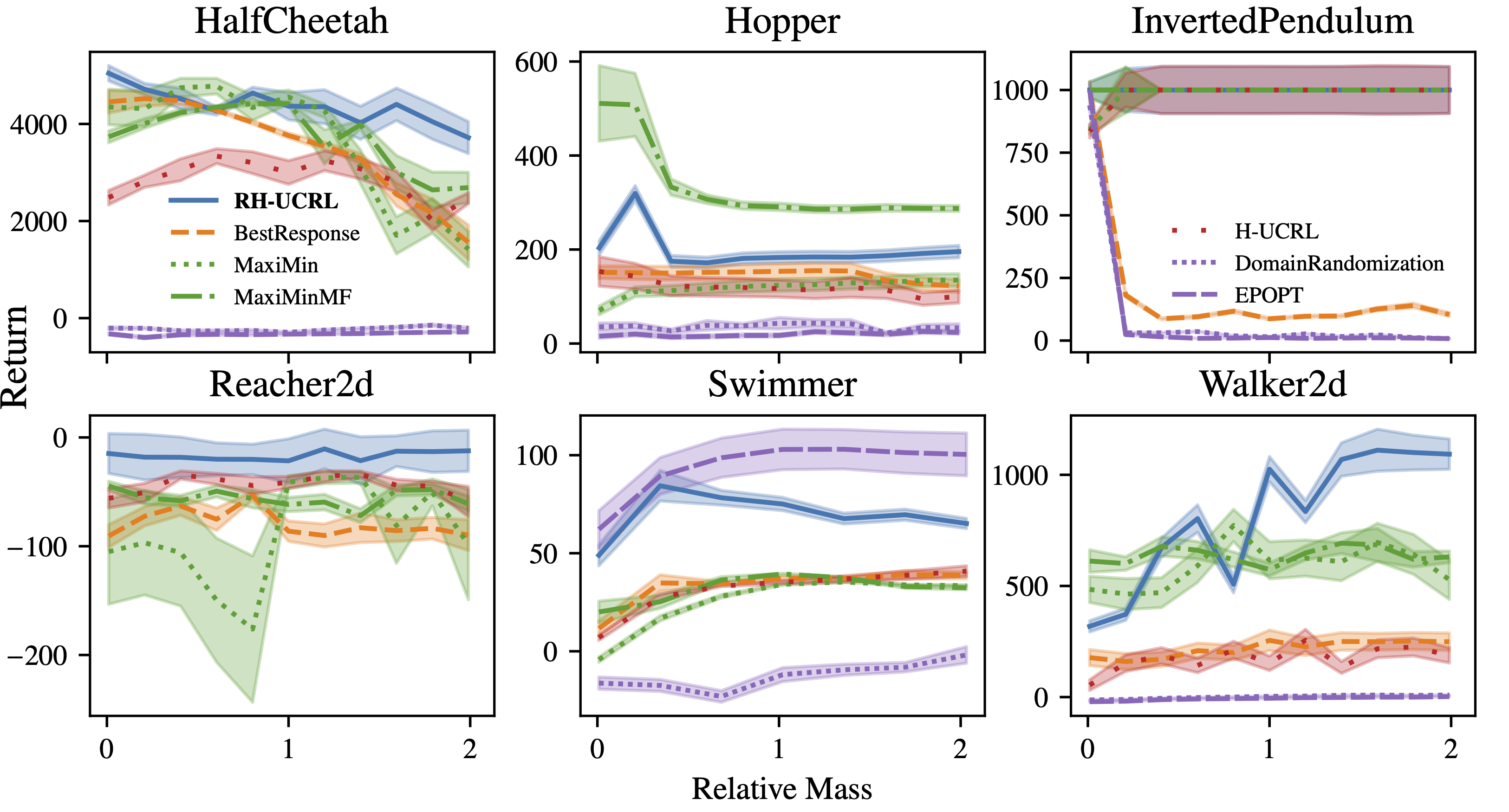
Baseline Comparison: We see that the performance of RH-UCRL is more stable compared to the other benchmarks and it is usually above the other algorithms. For the Swimmer environment, EP-OPT performs better, but in most other environments, it fails compared to RH-UCRL.

Ablation Discussion: In the inverted pendulum, best response has very bad performance for a wide range of parameters. This is because early in the training it learns that the hardest mass is the smallest one, and then always proposes this mass, and fails to learn for the other masses. As a non-robust ablation, H-UCRL constantly has lower performance than RH-UCRL. Maximin-MF and Maximin-MB perform similarly in most environments, except in the hopper environment.

Adversarial Robust Reinforcement Learning

The final experiment in which we tested RH-UCRL is in a truly adversarial RL setting: We first train a policy using the different algorithms and then we allow an adversarial a second training phase for this fixed policy. We refer to the performance of the policy in the presence of such adversary asthe worst-case return. Likewise, we refer to the performance of the policy without any adversary as the average return. This evaluation procedure is in contrast to what it is commonly done in the literature, in which an adversarial robust RL training procedure is employed, but only evaluated in the parameter-robust setting.

In the next figure we plot both metrics for the different algorithms previously discussed, as well as RARL (Pinto et al., 2017) and RAP (Vinitsky et al., 2020) baselines.

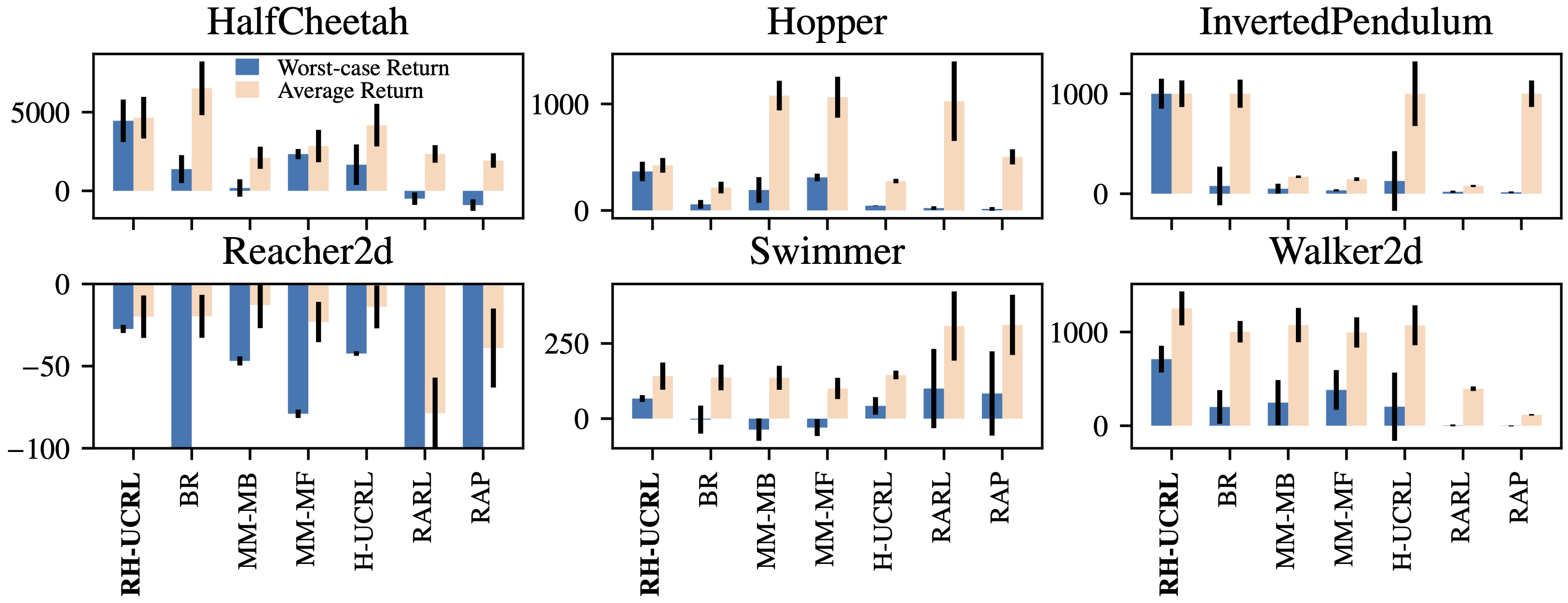
We first see that all algorithms have lower worst-case than average performance. However, the decrease of RH-UCRL performance is the least in all benchmarks. Furthermore, RH-UCRL usually has the highest worst-case performance, and also reasonably good average performance.

References

Chua, K., Calandra, R., McAllister, R., & Levine, S. (2018). Deep reinforcement learning in a handful of trials using probabilistic dynamics models. Neural Information Processing Systems (NeurIPS), 4754–4765.

Curi, S., Berkenkamp, F., & Krause, A. (2020). Efficient Model-Based Reinforcement Learning through Optimistic Policy Search and Planning. Neural Information Processing Systems (NeurIPS), 33.

Pinto, L., Davidson, J., Sukthankar, R., & Gupta, A. (2017). Robust adversarial reinforcement learning. International Conference on Machine Learning, 2817–2826.

Vinitsky, E., Du, Y., Parvate, K., Jang, K., Abbeel, P., & Bayen, A. (2020). Robust Reinforcement Learning using Adversarial Populations. ArXiv Preprint ArXiv:2008.01825.

Tobin, J., Fong, R., Ray, A., Schneider, J., Zaremba, W., & Abbeel, P. (2017). Domain randomization for transferring deep neural networks from simulation to the real world. International Conference on Intelligent Robots and Systems (IROS), 23–30.

Rajeswaran, A., Ghotra, S., Ravindran, B., & Levine, S. (2016). EPOpt: Learning Robust Neural Network Policies Using Model Ensembles. International Conference on Learning Representations, (ICLR).

Curi, S., Bogunovic, I., & Krause, A. (2021). Combining Pessimism with Optimism for Robust and Efficient Model-Based Deep Reinforcement Learning. International Conference on Machine Learning (ICML).

This post is based on the following two papers:

2021

Combining Pessimism with Optimism for Robust and Efficient Model-Based Deep Reinforcement Learning S. Curi, I. Bogunovic, A. Krause In Proc. International Conference on Machine Learning (ICML), 2021 [bibtex] [abstract] [pdf] [long]

2020

Efficient Model-Based Reinforcement Learning through Optimistic Policy Search and Planning S. Curi, F. Berkenkamp, A. Krause In Proc. Neural Information Processing Systems (NeurIPS), 2020 Spotlight presentation [bibtex] [abstract] [pdf] [poster] [code]