Learning as an Iterative Process
One key challenge that resonates in numerous learning tasks, is the process of deciding what to learn next. For example, imagine you are trying to learn a new hobby. One way to learn your hobby quickly, would be to keep track of a reading list of books that will allow you to learn from experts. As you keep reading these books from your reading list, you’ll need to decide which of them is worth investing time to cover all the learning material. For example, if your goal is learning chess, there’s no need to repeat a beginner’s book twice, when you can already progress to learning new opening tactics.
How can you intelligently choose the next book? Active learning algorithms can methodologically guide you in your learning endeavor.
Let’s take our chess learning problem and model it as an Active Learning problem. Suppose that each book can be represented as a set of features that uniquely identify it. Let’s also assume that you can freely order any book in Amazon Books, denote the set of all of these books as \mathcal{X} and assume that there exists some unknown function f(x) that maps features of books to your ability to win chess games. Let’s further denote our reading list, from which we “sample” new books, as \mathcal{S}. Classical Active Learning algorithms try to address the following question:
How can we globally learn f by sampling (noisy) observations of it within \mathcal{S}?
Uncertainty Sampling
So how can we use Active Learning to solve our chess learning problem? First, assume that at each round n the learner has to choose a book, represented by a point x_n \in \mathcal{S}. Given this choice, it observes a noisy measurement y = f(x) + \varepsilon(x) where \varepsilon is independent, but possibly heteroscedastic, noise. Deciding how to sample x_n (typically) depends on all previously collected data \mathcal{D}_{n -1} = {{\{(x_i, y_i)\}}_{i < n}}. In particular, \mathcal{D}_{n -1} = {{\{(x_i, y_i)\}}_{i < n}} is typically used to learn a stochastic process that models our probabilistic hypothesis over the function f.
.One classical method for Active Learning is “Uncertainty Sampling” [1]Lewis, D. D. and Catlett, J. Heterogeneous uncertainty sampling for supervised learning. In Machine learning proceedings 1994. Elsevier, 1994.. Uncertainty Sampling chooses the next query point by greedily maximizing the variance of a stochastic process that models f. More formally, we write x_n = \arg\max_{x \in \mathcal{X}}\mathrm{Var}[y \mid \mathcal{D}_{n - 1}]. Note that if we model f with a Gaussian Process, the computation of Uncertainty Sampling is exact, i.e., the variance after having observed \mathcal{D_{n - 1}} can be computed in closed-form.
A more modern view generalizes Uncertainty Sampling by taking an information-theoretic approach. Specifically, one can show that for homoscedastic noise, x_n = \arg\max_{x \in \mathcal{S}} \mathrm{I}(f_{\mathcal{S}}; y \mid \mathcal{D}_{n - 1}) reduces to the classical decision rule of Uncertainty Sampling.
When is Directedness Crucial?
We can spot two weaknesses of active learning and Uncertainty Sampling for our chess learning problem:
- Learning from every single book in Amazon Books is very impractical.
- Learning with Uncertainty Sampling is not directed towards learning chess, making it less suitable for choosing chess books.
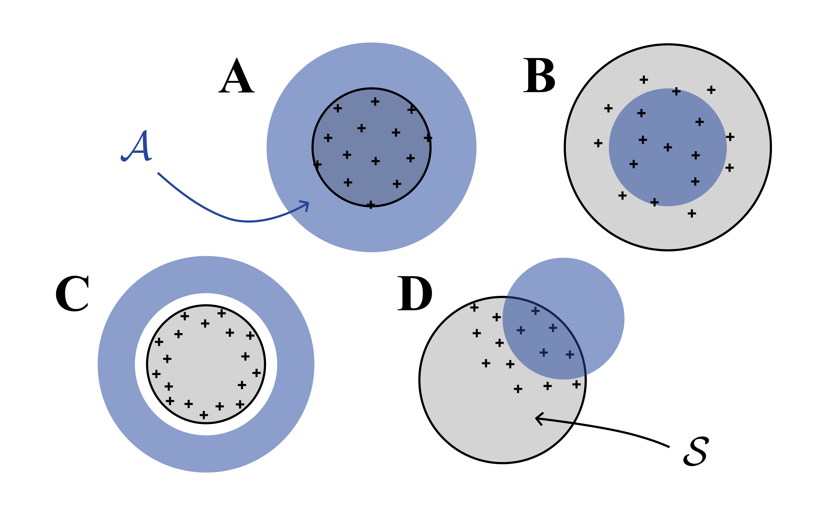
There is no need to read all the books in Amazon’s library. As mentioned before, some books are more relevant than others. In this case, we would want to choose an “area of interest” \mathcal{A} \subseteq \mathcal{X}, that can guide our learning. Note that we still haven’t specified whether \mathcal{A} \subseteq \mathcal{S} or not. While this difference may seem “innocent” at first, it raises some deep questions regarding the learner’s generalization. We’ll start with the easier case, where \mathcal{A} \subseteq \mathcal{S} (compare with case B below), and address the more challenging case \mathcal{A} \not\subset \mathcal{S} (C and D) later. In the meantime, can you think what makes it more challenging?

As we saw, Uncertainty Sampling is designed to learn about f globally and therefore does not address the directed case, in which we only care about a specific part of \mathcal{X}, thus learning f globally may be “wasteful”. What should we do to focus our learning in \mathcal{A} more effectively? Enter Information-based Transductive Learning (ITL)[2] Jonas Hübotter, Bhavya Sukhija, Lenart Treven, Yarden As, & Andreas Krause. (2024). Transductive Active Learning: Theory and Applications. . Compare \arg\max_{x \in \mathcal{S}} \mathrm{I}(f_{\mathcal{S}}; y \mid \mathcal{D}_{n - 1}) and \arg\max_{x \in \mathcal{S}} \mathrm{I} (f_\mathcal{A}; y \mid \mathcal{D}_{n - 1}). Although the two querying rules may appear similar at first glance, a closer examination reveals that they result in significantly different decision rules.
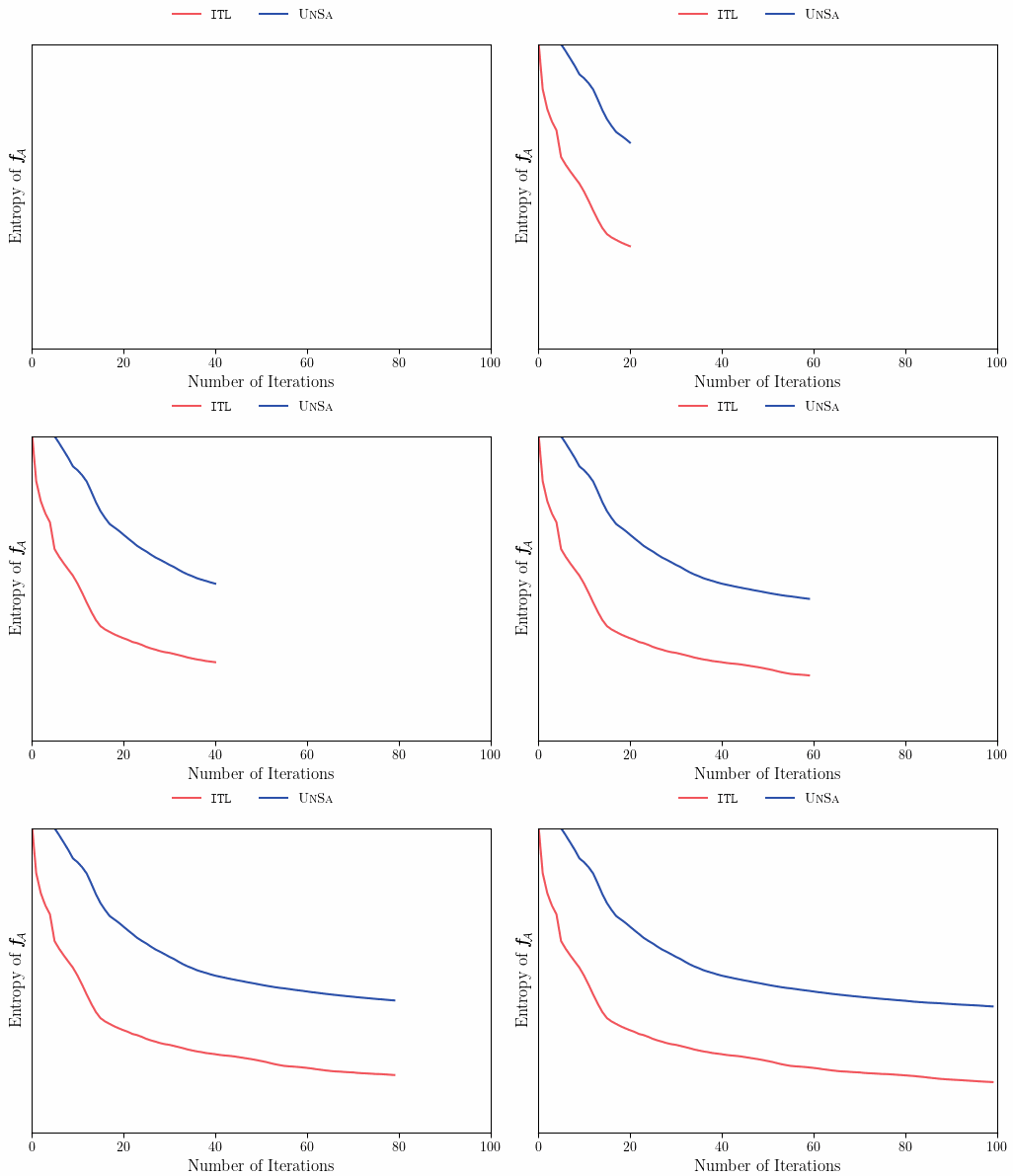
We can see that ITL takes one step further than Uncertainty Sampling, and computes the posterior distribution, given that our next query is in \mathcal{A}. This is in contrast to Uncertainty Sampling, which queries x_n based only on a prior distribution, that does account for our current specific knowledge of \mathcal{A}. One important fact about ITL, is that in the undirected case, where our “area of interest” is “everything” (\mathcal{S} \subseteq \mathcal{A}, case A above), under homoscedastic noise, ITL reduces to Uncertainty Sampling (can you think why?). Notably, in the undirected case, prior and posterior sampling are the same(!) but in the directed case they can be drastically different — allowing the learner to focus only on those books that are related to chess. The plot below illustrates how prior and posterior sampling differ in the directed case.


As we see, ITL’s decision rule samples points that reduce uncertainty in \mathcal{A}, leading to improved sample efficiency and better performance during learning and at convergence.
Extrapolation
In the previous section we saw how learners can focus on specific areas of interest within \mathcal{S} to learn more “personalized” tasks. An orthogonal, but equally important challenge, is concerned with problems that require learners to generalize and extrapolate outside of their direct training data.
To illustrate this, consider again our chess learning example. Since you only order books from Amazon Books, and you don’t speak Russian, you cannot be exposed to novel chess openings that only exist in Russian chess literature. How learning only from English books can still help you with playing against Russian-speaking players? How much should we expect to learn about Russian openings by only reading from English chess literature?
As we saw before, to some extent, classical active learning theory cannot cover cases in which the learner has to extrapolate outside of its accessible sample space. Such cases often arise not only due lack of access to data or distributional shifts, but also due to safety restrictions we want to impose on the learner (like “censoring books”). Therefore, we need more general tools to handle the aforementioned problems. As discussed before, the decision rule given by \arg\max_{x \in \mathcal{S}} \mathrm{I} (f_\mathcal{A}; y \mid \mathcal{D}_{n - 1}) does not make any specific assumptions on the relationship between \mathcal{A} and \mathcal{S}, and thus, it is general enough to tackle cases where generalization outside of \mathcal{S} is required. But how can we quantify generalization outside of \mathcal{S}?
In our recent paper, we derive a novel bound on the uncertainty of points x \in \mathcal{A}. In particular, it can be shown that this uncertainty is composed of irreducible and reducible parts, wherein the irreducible uncertainty can be written as \text{Var}[f(x) \mid f_{\mathcal{S}}]. Observe that even if the learner is given full knowledge of f at every point x \in \mathcal{S}, the irreducible uncertainty of points outside of \mathcal{S} will typically be non-zero. Importantly, irreducible uncertainty is a lower bound to the total uncertainty one can hope to reduce.
The good news are that learners can still gain information (and reduce uncertainty) by querying the “right” points in \mathcal{S}. How do you choose these points? One way is to use ITL, which, under some mild assumptions, guarantees that the reducible uncertainty will converge to zero.
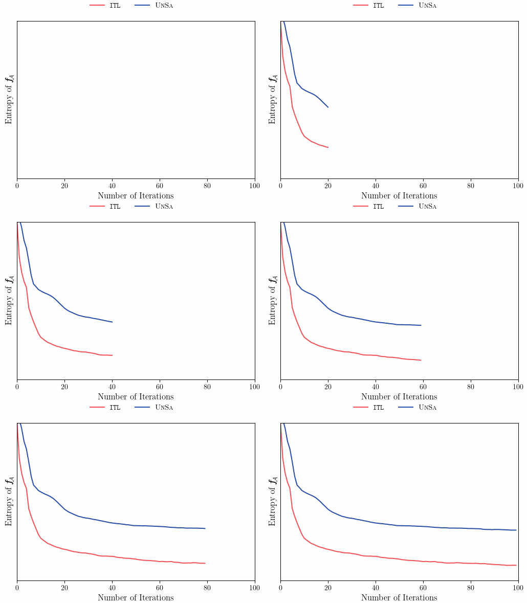
Let’s modify our previous example to a case that requires extrapolation outside of \mathcal{S}.


Like the previous example, ITL’s directedness towards \mathcal{A} allows it to sample more informative query points, leading to better performance, even when the learner has no direct access to \mathcal{A}.
Closing Thoughts
Our chess learning example demonstrates two crucial aspects of intelligent learning: the ability to focus only on what’s important for the task or goal at hand (“no need to read cooking books if you care about chess”) and the ability to generalize outside of the accessible data (“learning Russian chess openings from English books”).
ITL brings a fresh perspective to deal with these challenges. By following a principled information-theoretic approach, we are able to derive a decision rule that is theoretically sound (i.e., does not rely too much on heuristics), has convergence guarantees, and finally, exhibits strong empirical performance.
For more details about this work, further experiments on harder problems (quadcopter safe exploration, neural-network fine-tuning) check out our recent arxiv and workshop papers.
Footnotes

