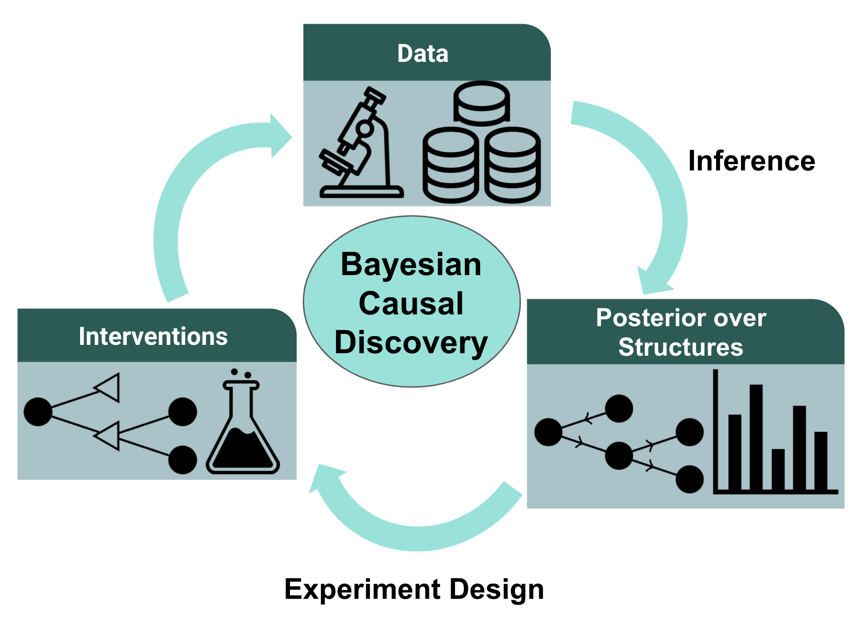
Figure 1: A workflow for a Bayesian approach to causal structure discovery. In two recent works from our lab, we study the inference and experiment design components of the pipeline.
Causal Inference and Machine Learning
Causality and machine learning have been studied largely independently, but recently there has been significant excitement in the intersection of both fields. One hope is that by inferring causal rather than statistical dependencies, we might be able to design systems that can perform robustly outside of the training environment.
Causal discovery refers to the task of inferring the explicit causal relations among a set of random variables. Currently, many causal discovery algorithms are designed under strong assumptions that may not hold in the complex domains causal discovery is most frequently deployed in e.g., economics, health care, biology. These limitations range from assumptions about the underlying causal system to assumptions about the data collection pipeline.
A Real-World Application: Gene Regulatory Networks in Systems Biology
Let’s look at the task of causal discovery by way of the following example: gene regulatory networks (GRNs). Inferring GRNs from gene expression data is a common use case for causal discovery in practice. A GRN may look like the network shown below.
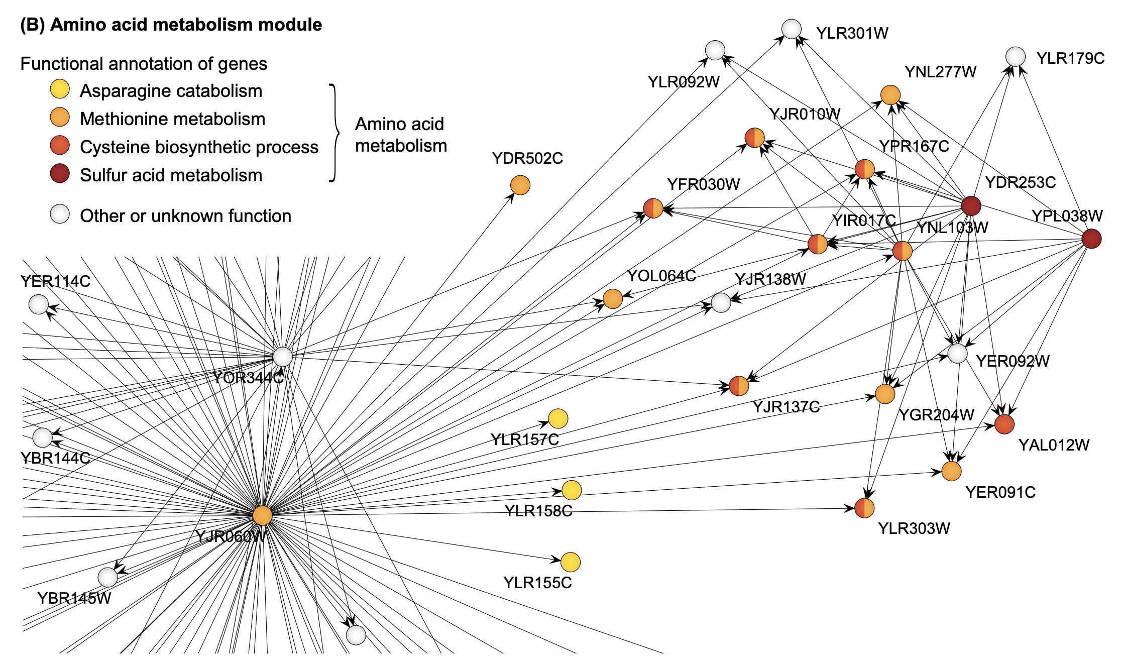
Figure 2: Example gene regulatory subnetwork extracted from a yeast gene network (taken from Marbach et al., 2009).
Unfortunately, many existing causal inference algorithms are disconnected from the requirements to successfully apply them in this case.
- Causal inference methods (like the PC algorithm or GES) compute a point estimate of the causal graph. For GRNs and other real-world applications, we often have limited data but a lot of causal variables. We need to accurately quantify the uncertainty in the inferred graph structure, in particular for experiments that affect health care or the safety of humans.
- Causal inference algorithms most often assume simplistic linear or categorical models. Real GRNs evolve as systems of coupled differential equations over time. In GRNs, we can measure the genes’ steady states and reason about the effects of interventions, but their dependency could be highly nonlinear. [1]As for instance captured by these GRN simulation models.
- In practice, and when inferring GRNs, we commonly consider online streams of experiments. Experiments are costly in terms of time and resources, and thus we need to design informative experiments in the form of interventions, also termed experiment design, to maximize the discovery of causal structures within an experimental budget.
- Experiment design algorithms often assume single intervention targets. Conversely, for GRNs, it is now possible for experimenters to perturb multiple genes at once, saving massive amounts of time and resources in the scientific experiment cycle.
In two recent NeurIPS 2021 papers that both resulted from master’s theses of our group, we study two aspects of the above causal inference pipeline, to move towards causal discovery with less restrictive and simplistic assumptions in real applications such as GRN inference. First, we will look at how we can infer more complex and realistic structural models given a data set of observations. After, we consider the experiment design pipeline and how we can select batches of interventions to maximize knowledge of the causal structure given a fixed experimental budget.
Notation
Let us formalize the ideas from the introduction. Given a data set of observations D = \{x^{(1)}, \dots, x^{(N)}\}, our goal is to discover the causal directed acyclic graph (DAG) G and parameters \Theta that model the causal generative process of the data. In general, G cannot be completely identified using only observations D . The graph can only be identified up to its so-called Markov equivalence class (MEC), where certain edges in the DAG skeleton are not directed. Figure 5d gives an example of all members of a MEC for a specific 5 variable tree graph. Figure 5a shows the compact representation of this MEC using undirected edges. In both works presented here, we assume causal sufficiency: that no two variables share an unobserved common cause.
A (hard) intervention do(x_i := c) sets the value of x_i to c in the generative process, effectively disconnecting variable i from all its natural causes when sampling a joint observation. If c is random, this is akin to a randomized control study. To fully identify G , we require interventional data when intervening upon specific target nodes. The book by Judea Pearl and the book by Jonas Peters et al. give a more formal introduction to causal inference.
Bayesian Structure Learning for More Complex Models
As discussed above, in practical applications such as GRN inference, we usually do not have sufficient data \lvert D \rvert to be certain about G or even its MEC. Thus, we may be interested in inferring a Bayesian posterior
In a recent NeurIPS 2021 paper of our group, we propose an efficient, fully differentiable inference framework for inferring Bayesian posteriors over structures (“DiBS”) of the above form. Specifically, by being able to infer p(G, \Theta | D) , i.e. G and \Theta jointly, we are no longer limited to inference of models where the marginal likelihood
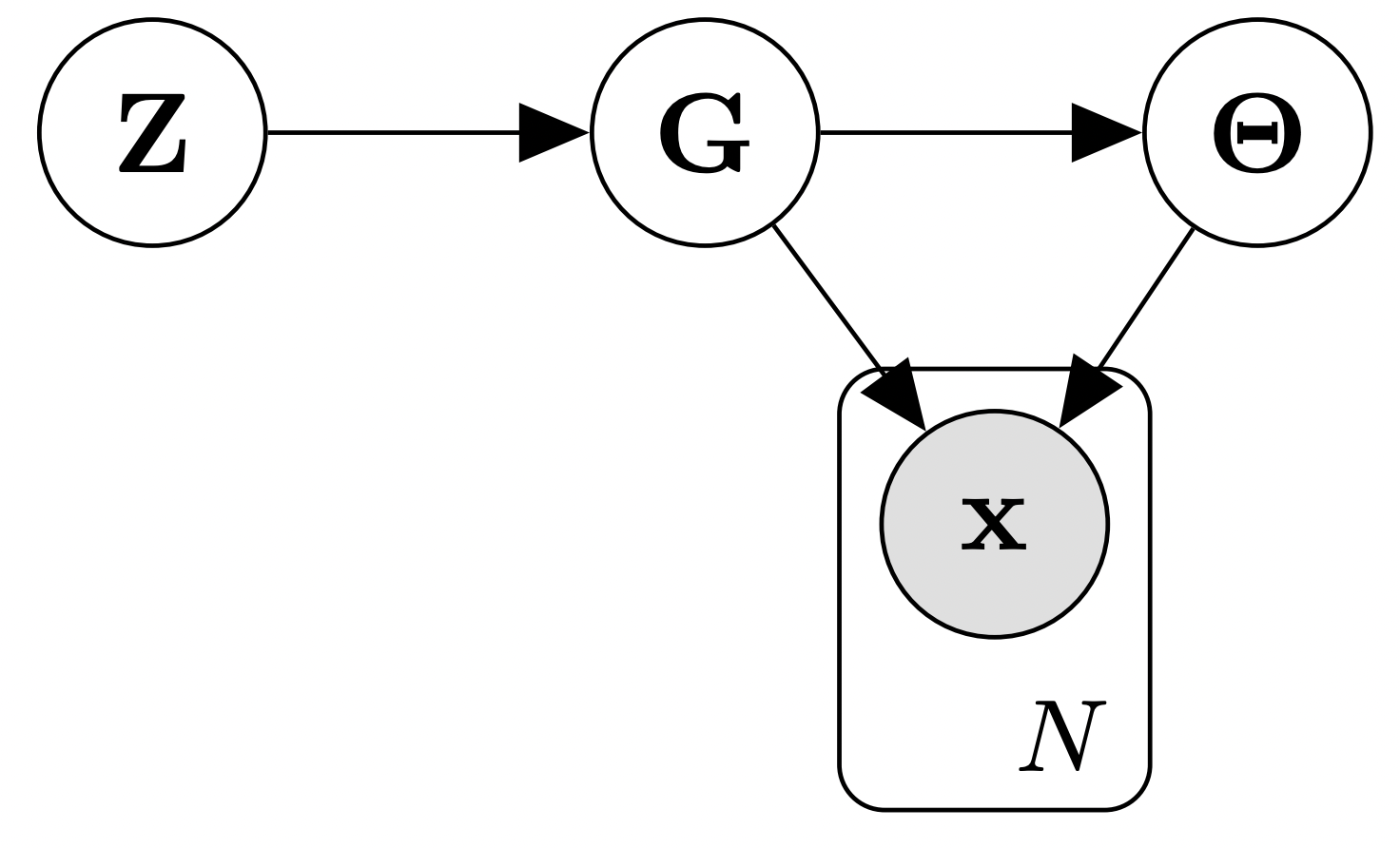
Figure 3: Generative model with latent variable Z , generalizing the standard Bayesian setup where only G , \Theta , and x are modeled explicitly.
Our key insight is the following: By assuming, without loss of generality, that a latent variable Z governs the generative process of the DAG G , we can translate the inference task over the discrete posterior p(G | D) into an inference problem over the continuous latent variable Z :
We can thus solve our original problem by inferring the continuous posterior p(Z | D) instead. In our paper, we show how to define p(Z) and p(G | Z) to ensure that we only model valid directed and acyclic graphs G . We furthermore provide expressions for REINFORCE and Gumbel-softmax-based estimators for the scores \nabla_Z \log p(Z | D) .[2]Whether or not we are able to apply the lower-variance Gumbel-softmax reparameterization estimator depends on whether or not the (marginal) likelihood p(D | G) or p(D | G, \Theta) have a … Continue reading This allows us to use any general-purpose and gradient-based inference method to ultimately infer p(Z | D) . In our work, we use Stein variational gradient descent (SVGD) to do the job, but in principle, one could also consider methods like, e.g., Hamiltonian Monte Carlo (HMC) or Stochastic Gradient Langevin Dynamics (SGLD).
Figure 4 below visualizes an example of what inference with DiBS looks like when using SVGD as the black-box inference method. For further details on DiBS, check out our paper and the corresponding GitHub repository with code and an example notebook used to generate Figure 4.
Figure 4: DiBS with SVGD for inference of p(G, \Theta | D) for synthetic data from a linear Gaussian model. The top shows the true adjacency matrix G . Below are the matrices of edge probabilities modeled by the particles Z (here 20) that are transported by SVGD to approximate the posterior.
Having considered the graph and parameter inference part of the causal discovery pipeline, we will now look at the optimal experiment design process, and specifically how we can select near-optimal batches of interventions to maximize knowledge of the causal structure given a fixed experimental budget.
Experiment Design for Batched Multi-perturbation Interventions
Observational data is often not enough to uniquely identify a system’s causal structure. In fact, without making assumptions on the structural causal model, even infinite observational data is only enough to identify a causal structure up to its Markov equivalence class. In some settings, experiments can be performed on the system to improve identifiability.
For learning gene regulatory networks, it is possible to perform large batches of experiments concurrently. This setting motivates a second paper of our lab presented at NeurIPS 2021. Much prior work in this domain designs batches where each experiment intervenes on a single variable. However, it is possible in single-cell biology experiments to intervene on multiple variables for a single cell. Motivated by this technology, we tackle the problem of how to select batches of multi-perturbation interventions. We use the term perturbation to describe the change to a single variable in an intervention on multiple variables.
Concretely, we consider designing a batch of multi-perturbation interventions \xi = \{I_1, I_2,\ldots\} . We constrain both the batch size \lvert \xi \rvert \leq m and number of perturbations per intervention \lvert I\rvert \leq q . To motivate our algorithm, we consider a simplified setting with arbitrarily large amounts of observational data, and arbitrarily large amounts of data for each unique intervention (noiseless interventions). We will see that even with these simplifications, the task of experiment design in this setting is still very challenging. We will also see in experiments that our algorithm, developed under these assumptions, performs well in settings with finite samples. We aim to select \xi to maximize
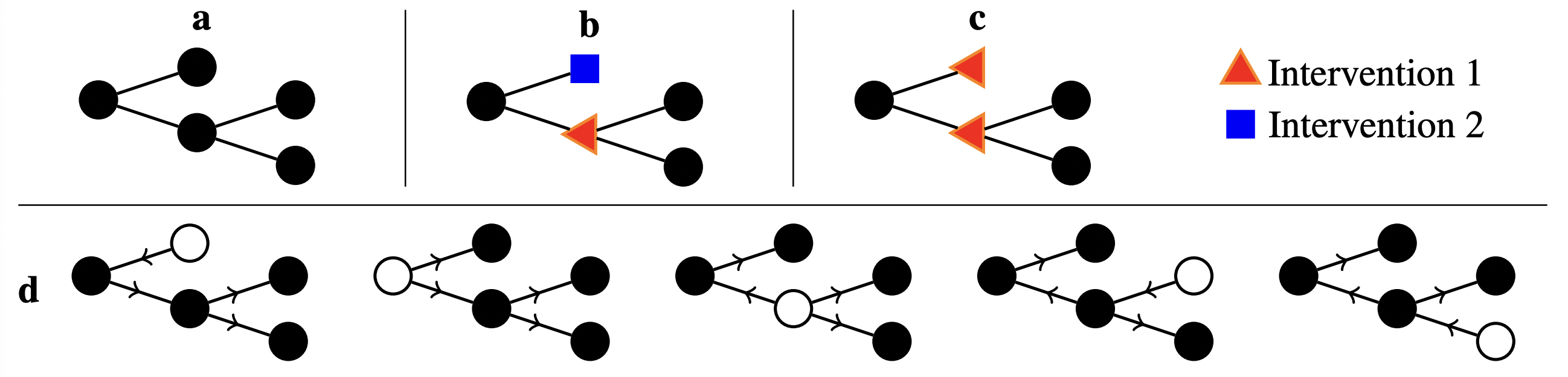
Figure 5: a) a representation of the MEC for a 5 variable system with a tree causal structure. b) two separate single perturbation interventions that fully identify the causal structure given arbitrary numbers of samples. c) a single multi-perturbation intervention that also fully identifies the causal structure. d) all members of the MEC enumerated, each corresponding to a different root node marked in white Such a correspondence is specific to tree structures.
We demonstrate that multi-perturbation interventions can result in much faster identification of the causal structure. An example of this is illustrated in figure 5b and 5c. However, designing such experiments is difficult because we must select interventions over a very large search space: a batch of multi-perturbation interventions is a set of sets. Moreover, two nearby perturbations within the same intervention can interfere, reducing their effectiveness. These interactions need to be accounted for when designing experiments.
Since we maintain a probability distribution over possible graphs, we can simulate the expected objective value for a given batch before actually performing the experiment. Designing an efficient algorithm boils down to two problems.
- Efficiently simulating our objective. For F_{\text{EO}} a naive approach would take exponential time in the number of variables since the MEC can contain number of graphs exponential in the number of nodes.
- Selecting a batch which achieves high objective without enumerating all possible batches.
In \mathcal{O} \left( m^4 p^{5/2}/\epsilon^3 \right) evaluations of R , our algorithm achieves a solution \xi such that
Our algorithm selects a batch by starting with an empty batch and then using a stochastic continuous subroutine to near-greedily select multi-perturbation interventions until the batch size limit is reached. It tackles the two problems listed above by
- The stochastic continuous subroutine selects interventions by sampling elements from the sum in F_\text{EO} , so that the objective never needs to be computed exactly.
- To show that this algorithm can achieve the near-optimality guarantee above, we use results from submodular optimization. These guarantee that the stochastic continuous subroutine corresponds to near-greedy intervention selection, and that this in turn leads to a near-optimal batch.
In experiments, our algorithm performs favorably compared to two baselines: a strong single-perturbation baseline and randomly selected multi-perturbation experiments. Two key settings we explore in our experiments are:
- Synthetic experiments where we obtain only finite samples per intervention, demonstrating that our theory in the noiseless intervention setting motivates a high-performing practical algorithm.
- Synthetic experiments where the ground truth DAG is a real gene regulatory subnetwork, demonstrating that our approach performs well in realistic DAG structures.
Please check out our paper for further details on the algorithm design and experiments.
Outlook
The intersection of causality and machine learning is an exciting research area that we think could have a great impact on science and engineering. There are many discoveries to still be made in this direction. In our two works outlined above, we only consider systems no with unobserved confounding, i.e., where all variables that affect more than one variable are observed. Moreover, to fully harness its application in practice, we need to improve the scalability of causal discovery and experiment design methods to more than hundreds or even thousands of variables, e.g. in modern GRN inference tasks.
We’ll be at the NeurIPS poster sessions if you would like to learn more about the two papers. The differential Bayesian structure learning poster will be at 17:30-19:00 Zurich time on Tuesday 7th December. The multi-perturbation experimental design poster will be at 9:30-11:00am Zurich time on Thursday 9th December.By Lars Lorch and Scott Sussex
December 6, 2021
This post is based on the following two papers:
2021 | |
| |
| |
Footnotes
| ↑1 | As for instance captured by these GRN simulation models. |
|---|---|
| ↑2 | Whether or not we are able to apply the lower-variance Gumbel-softmax reparameterization estimator depends on whether or not the (marginal) likelihood p(D | G) or p(D | G, \Theta) have a well-defined gradient with respect to the adjacency matrix of G . The REINFORCE estimator always applies. |