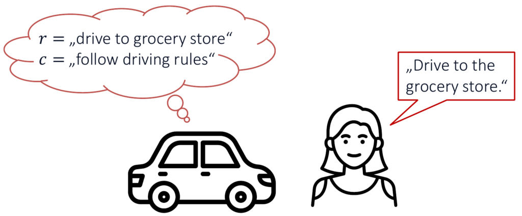
Human preferences often naturally decompose into rewards and constraints. For example, imagine you have an autonomous car and tell it to drive you to the grocery store. This task has a goal that is naturally described by a reward function, such as the distance to the grocery store. However, other implicit parts of the task, such as following driving rules or making sure the drive is comfortable, can be naturally described as constraints.
A key challenge for deploying AI systems in the real world is to ensure that they act “in accordance with their users’ intentions’’ – that they do what we want them to do. The most common way of communicating to an AI system what we want it to do is through designing a reward (or cost) function. However, in practice, it is challenging to specify good reward functions, and misspecified reward functions can lead to all kinds of undesired behavior.
Instead of designing reward functions explicitly, we can try to learn the task from humans. For example, in reward learning we learn a model of the reward function from human feedback, such as pairwise comparisons of trajectories, and then use standard RL algorithms to optimize for this learned reward function.
Reward functions are not the only way tasks are specified in RL. In practical applications, such as robotics, alternative ways of specifying tasks are often more useful, for example constraints or goal states. Based on our recent ICML 2022 paper, this post argues that reward models might not be the most effective way of representing learned task specifications in all situations. In particular, we find that learning constraints can be a more robust alternative, and we provide a concrete formulation of learning about unknown preference constraints.
Why learn constraints?
Let us consider an example to understand why we might want to represent tasks as constraints in addition to or instead of reward functions. Let’s say we want to train a policy to drive a car. To illustrate this, we consider a simplified driving simulation, introduced initially by Sadigh et al. 2017: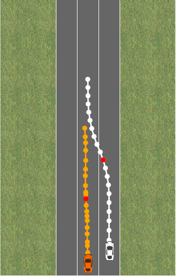
In this environment, we want to control the orange car while the white car moves on a fixed trajectory. We want our car to drive at a target velocity v_0 while staying on the road and, importantly, not getting too close to the other car. It is natural to decompose this task into a reward – how close are we to velocity v_0 – and constraints – for example, “stay on the street” or “don’t get too close to the other car”. Let’s say each policy \pi is described by a feature vector f(\pi) \in \mathbb{R}^d and we have a linear function \theta^T f(\pi) that describes the reward and a linear function \phi^T f(\pi) than encodes the constraints.
If we wanted to encode the task as a single reward function, it would be natural to choose
and then aim to find \pi^* \in \text{argmax}~ r(\pi). Instead, we could encode the task as a constrained optimization problem and aim to find
for some threshold \tau. At first glance, it might seem like these are equivalent. We can express the constrained optimization problem as an unconstrained optimization problem with a penalty. And indeed, both of these approaches give reasonable behavior for the driving task:
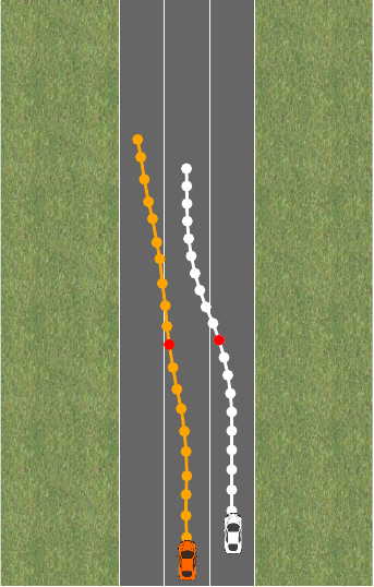
Say we now want the car to pull over to the side of the road instead of driving at a target velocity. We will have a different reward \theta, but the same constraints \phi. Let’s try to swap out \theta in both the pure reward and the reward plus constraint formulation:
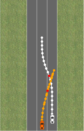
Why does only the policy optimized for the constrained problem pull over as we want it to? In the pure reward formulation, the penalty term is too large and regularizes too strongly. We’d have to choose a smaller \lambda to get good behavior in this situation. In a sense, the constraint formulation is more robust here because it does not require any additional tuning.
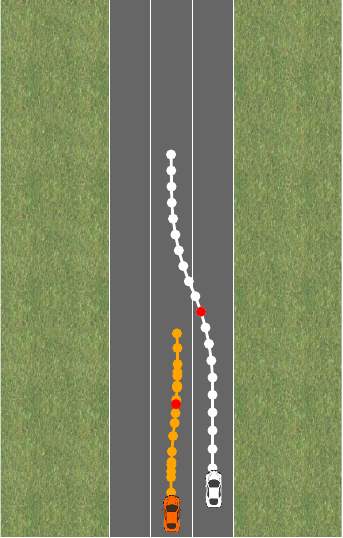
Something similar can happen when there are changes in the environment. Say the street is now blocked by three cars, and we want to again drive at target velocity v_0:
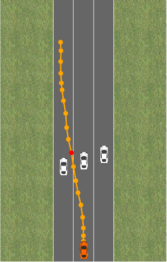
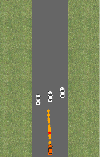
Now, it turns out that the reward penalty is too small, and we’d have to choose a bigger \lambda to avoid crashing into the other cars. The constraint formulation still works because crashing into the other cars is simply infeasible.
This example motivates why constraint task formulations are useful in general. When the full task specification is unknown as for driving a car, the decomposition into rewards and constraints has another advantage: often, we know the reward component of a task, for example, where we want our car to drive, but not the constraint component of a task, for example, we cannot list out all explicit and implicit driving rules in a robust form.
Therefore, we focus on the situation where we know \theta but don’t know \phi. We assume we can ask an expert about \phi and make noisy observations about whether a trajectory is feasible or not.
Learning constraints in linear bandits
We want to study how we can learn about an unknown constraint from noisy feedback. In practice, this feedback would likely come from human experts, which is very expensive. Hence, we are particularly interested in being sample efficient. We choose to model this situation as a linear bandit problem, which is a helpful abstraction for studying exploration problems with a linear structure. However, existing work primarily focuses on the case where we want to learn about a linear function we want to maximize, while our problem is about linear constraints.[1]There is also some recent work on linear bandits with constraints which is different from our setting in various ways. For details, refer to the discussion in the full paper. So, we’ll have to adapt the standard linear bandit setting.
To adapt common bandit terminology, we say we have a finite set of arms \mathcal{X} \subset \mathbb{R}^d, where each arm could represent one policy controlling the car in our previous example. Our goal is to find
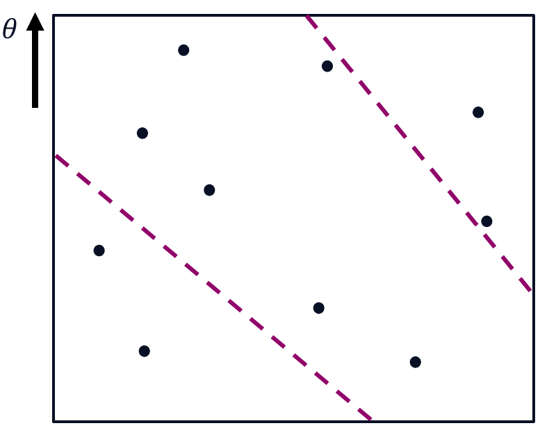
\phi is unknown but \theta is known. We consider a pure exploration problem, so we have two phases in which we first select arms to learn about \phi, and then recommend a solution in the second phase. We want to ensure we need as few samples as possible before we can decide which arm is optimal. Here is a 2D illustration of the setup:
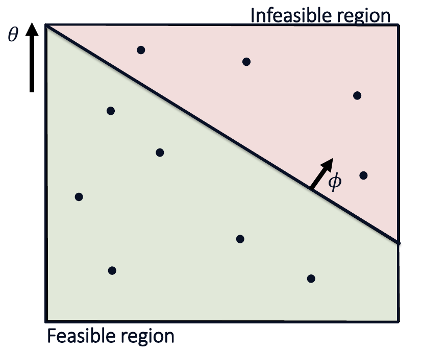
In our previous example, each arm would correspond to one policy, and arms get better along the y-axis. We want to find the best constrained arm. But, because we are uncertain about the true constraint boundary, we have to estimate it using confidence intervals. For example, we might only know that the true constraint boundary lies within a given region:
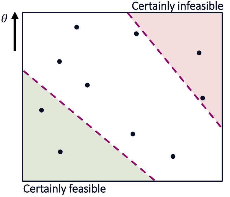
Additionally, we can consider the arm with the highest reward among the certainly feasible arms. This arm is our current candidate solution. Importantly, we know that all arms with less reward are suboptimal. The remaining arms are arms that could still be optimal:
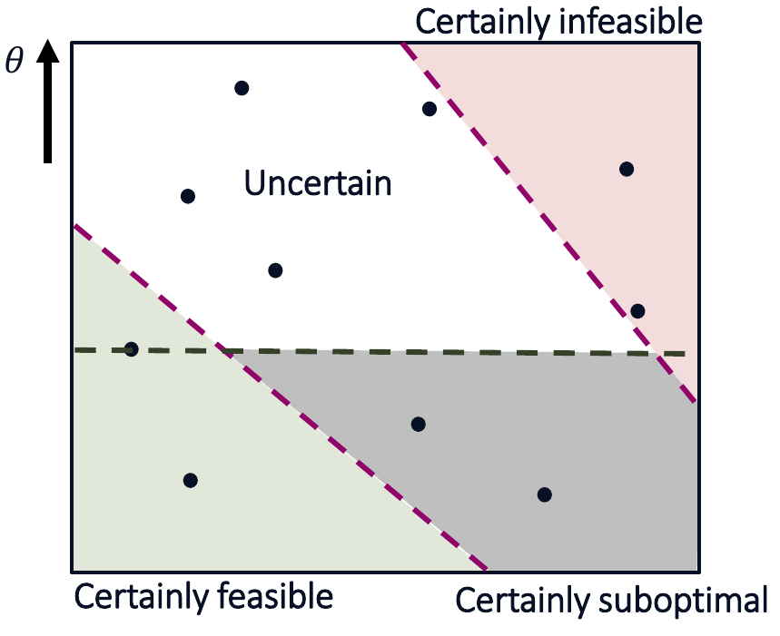
This insight allows us to design an active learning algorithm that reduces the uncertainty about these plausible optimizers and shrinks this set until it can identify the constrained optimal arm with high probability. We call this algorithm Adaptive Constraint Learning (short ACOL).
In our paper, we theoretically analyze this problem’s sample complexity and the algorithm. We provide a lower bound for the constrained best-arm identification problem and a sample complexity bound for Adaptive Constraint Learning.
The sample complexity of a problem depends on d / C_{\text{min}}^2 where C_{\text{min}} is the distance of the closest arm to the constraint boundary. So, a problem is more difficult if it has a higher dimension d or arms closer to the constraint boundary. ACOL matches this sample complexity in the worst case and even almost matches a problem-dependent sample complexity bound that we arrive at after a more careful analysis.
Empirical results
We can also evaluate Adaptive Constraint Learning (ACOL) empirically. We again use the driving environment but now implement the situation where we know \theta but do not know \phi. Instead, we can get noisy binary feedback from a simulated expert that tells us if a given policy is feasible or not. We need to identify the best feasible policy from a fixed set of pre-computed policies. By using well-calibrated confidence intervals, most methods will eventually find the correct solution, but we are interested in how many samples different methods need.
Hence, we evaluate the number of samples for finding the best policy and compare our algorithm ACOL to various baselines. Here is a simplified plot comparing ACOL to uncertainty sampling, a more naive active learning method, and uniform sampling:
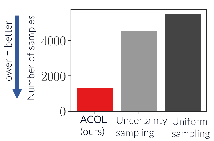
ACOL needs much fewer samples because it aims to make the most informative queries for finding the correct optimal policy. In our paper, we provide many more experiments in different environments. These give a more detailed picture, but the general message is the same as this single result: ACOL is more sample efficient than alternative methods when learning about unknown constraints.
In this post, we made two crucial observations. First, learning constraints and reward functions might help to make RLHF more robust. And second, we can adapt active learning techniques for reward learning to this constraint learning setting and still achieve strong theoretical results and good empirical sample efficiency. In the future, we hope to apply these methods to more practical applications and investigate if learning constraints is a valuable addition to learning rewards.
If you want to learn more about this work, read the full paper, or watch the pre-recorded presentation. If you are visiting ICML in-person, you can visit us at poster session 5 track 2 on Wednesday, 20 July, from 6:30 PM to 8:30 PM EDT.
This post is based on the following paper:Conclusion
2022